Automatically detect the perimeter of a city given an aerial or satellite image of the city. A convolutional neural network is used to identify the road network in the image, and then image processing techniques expand the road network into a contour of the city.

Figure 1. Diagram of detection method. a) Aerial image containing Lake Havasu City, AZ. b) Road network prediction from a CNN. c) Mesh surrounding the city after morphological operations to expand the road network. d) Contour of the largest mesh object overlaid on the original aerial image.

Overview

The process for perimeter extraction (see Figure 1) is largely inspired from this paper. In it, the authors construct Google Maps-esque images of cities using freely available Open Street Map (OSM) data. The road networks in these images are detected with elementary image processing techniques, and morphological operations expand the road networks into binary masks that encompasses the cities. A simple contour procedure around these masks produce the perimeters.

In this project, we accomplish the same perimeter detection task but with aerial images instead of artificial Google Maps-esque images. The overall scheme is essentially the same: identify the road network and apply morphological and contour operations to create a bounding perimeter. Indeed, the morphological and contour operations shown in Figure 1 are basically identical in the reference paper. The significant difference comes in the road detection step.

In the reference paper, road detection was relatively simple as the authors were able to choose specific colors for roads when constructing the synthetic images. Thus, road detection could be easily accomplished by filtering for colors or even with edge detectors operating on relevant color channels. Such techniques are not sufficient for road detection in aerial images as the source is not so nice: roads can vary in color and may blend in with their surroundings, and edge detectors will pick up noise such as buildings or natural scenery. Thus, a more sophisticated method is necessary.

Other work has shown that machine learning can be successfully used for road detection and the more general task of image segmentation. Here we use a convolutional neural network (CNN) with a modified U-Net architecture to perform road detection on aerial images. Training and benchmark data is generated via OSM road labels.

The results of the procedure for 5 Arizona cities (Bullhead, Flagstaff, Globe, Lake Havasu City, and Yuma) are presented and discussed in the Results section. Some suggestions for future improvement are offered in the Conclusion section. The outline for data acquisition, CNN training, and perimeter extraction procedure are detailed in the Methods section.

Full source code is available on GitHub.

Results

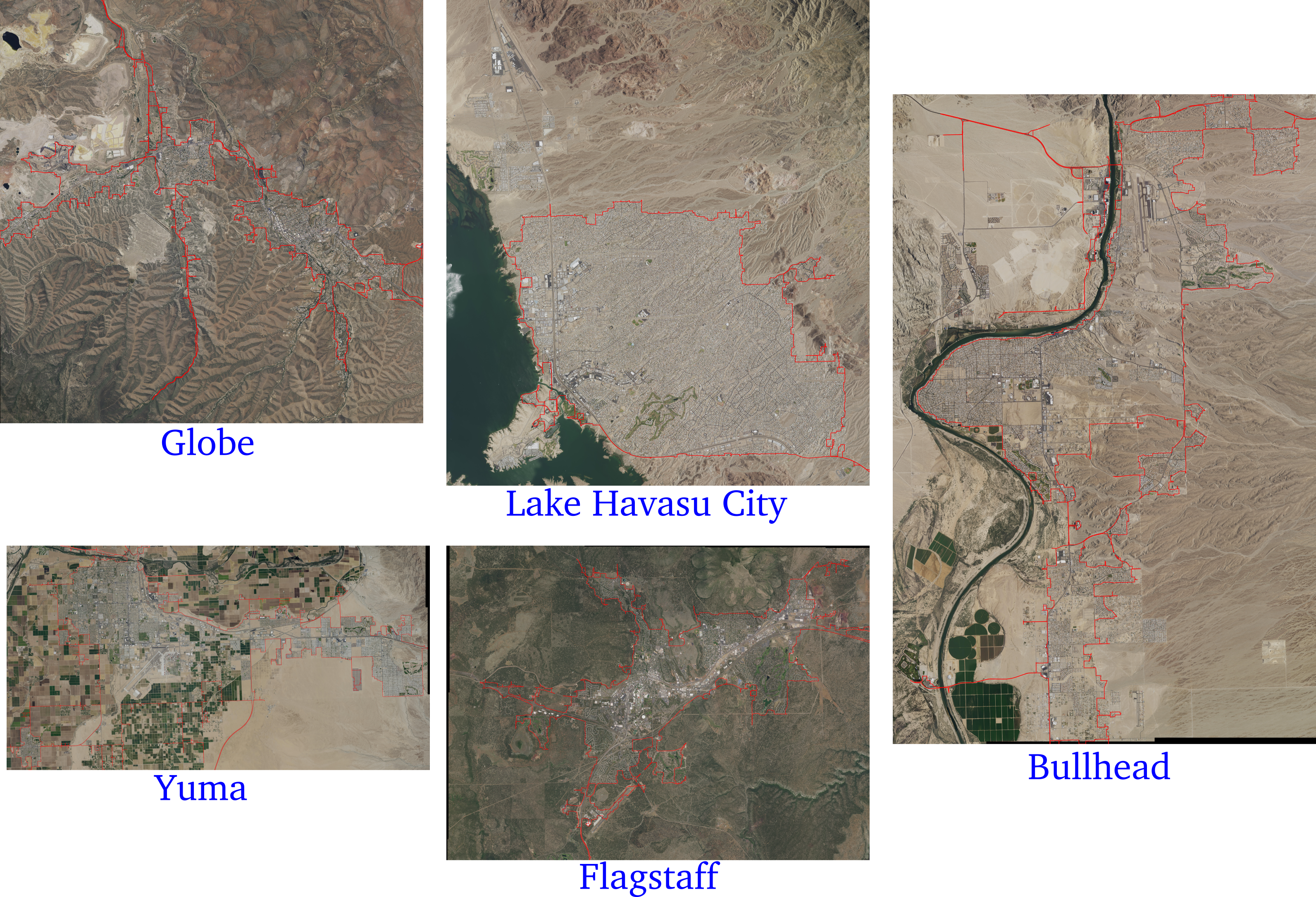
Figure 2. (Click to see full size) Results of perimeter detection process applied to five Arizona cities.

The outputs of the procedure applied to five cities are shown in Figure 2.

The detected perimeters approximate the cities very reasonably although some are better than others. Lake Havasu City and Flagstaff visually appear to be the best approximations with the contours closely following the extent of urban development. In Havasu, the areas on the top-left that are not part of the contour are in fact also not part of the city, so the algorithm was able to discriminate between cities or unincorporated communities if there is sufficient separation between them. However, the smaller island in the bottom left corner was not sufficiently detected despite being part of the city as the road network there is sparse. This suggests the algorithm struggles with significant patches of natural scenery not surrounded by roads.

The natural scenery also presented some problems in Yuma and Bullhead. In both cases the contours essentially encompass the city boundary, but there are additional patches of undeveloped land that could arguably be left out to form a tighter perimeter. This issue is exacerbated in Yuma which has a significant agricultural presence on the outskirts. The separations between crops fields are often partially miscategorized by the CNN as being roads resulting in some of the crop fields being part of the road network and thus within the contour.

Despite its somewhat disjointed structure, the detection algorithm performed quite well on Globe. The most obvious artifact of the detection method here are the very narrow segments in the north and south. These segments are part of the city, but the algorithm sometimes fails to capture the full extent of these areas likely because there are only a few roads present. It is also worth nothing that in the very left of the image, the detected perimeter actually encompasses another town and two unincorporated communities. Because these communities essentially bleed into Globe without any separation, the algorithm defines them as a single entity.

Conclusion

A procedure for automatically detecting city perimeters from aerial images was developed and tested on five cities in Arizona. The algorithm generally produced visually sensible perimeters with the boundaries entirely or almost entirely encompassing the cities. In many cases the detected boundaries closely aligned with the extend of urban development and thus produced a tight perimeter.

The two most significant challenges for the algorithm stem from natural scenery and multiple municipalities packed closely together. If multiple municipalities are packed together without any natural separation as with Globe, AZ and surrounding territories, the algorithm detects these as a single connected region. Manually specifying the limits of the city beforehand in the aerial image before applying the algorithm could alleviate this problem at the cost of requiring more human input; still, it is less effort than having a human trace the whole perimeter extent.

The natural scenery problem can result in over- or underestimation of perimeter boundaries. If natural scenery is part of the city but has few surrounding roads, it will not be detected in the road network and thus will not appear in the boundary. However, some specific scenery such as separation between farming crops (see Yuma in Figure 2) are often mistaken for roads by the CNN and thus erroneously included in the road network. The capability of the CNN to discriminate between these errors and true roads would mitigate this problem and could possibly be achieved by training on a larger dataset that includes more crops and natural scenery.

Methods

This section details the procedure for this project from data acquisition to CNN training to application. Full source code is available in individual Jupyter notebooks on GitHub with one notebook per subsection below (individually linked in the headers)

All computations were performed on a desktop computer with an Intel i5 6600K processor, 16GB of RAM, and an Nvidia 1070ti GPU.

Dataset

The georeferenced aerial images are sourced from the US National Agriculture Imagery Program (NAIP) which generated 1-meter-per-pixel aerial images of the entire US region. The data is freely available on an Amazon Web Services (AWS) S3 bucket (bandwidth fees apply if you are not in the US-East region).

For this project we focus on cities in Arizona. In particular, aerial images for Phoenix, Bullhead, Lake Havasu, Flagstaff, Globe, and Yuma are downloaded.

A single NAIP image covers only a small portion of land (based on the USGS quadrangle specification), so for each city multiple images must be downloaded. The Google Maps’ geolocator service is used to determine an appropriate bounding box for each city, and then NAIP images are downloaded to cover the entire bounding box.

Labels

Freely available OSM data is used to label the roads in all the images downloaded in the previous section. OSM provides shapefiles which contain line geometries for roads throughout the world. The latitude, longitude coordinates of the roads are matched to the georeferenced aerial images to produce binary mask images where pixels are labeled 1 if they contain a road and 0 otherwise.

However, OSM road geometries correspond to road centers rather than the full width of the roads. To compensate, road labels are expanded with a 3x3 kernel dilation operation applied twice (see Figure 3).

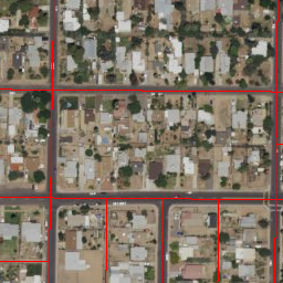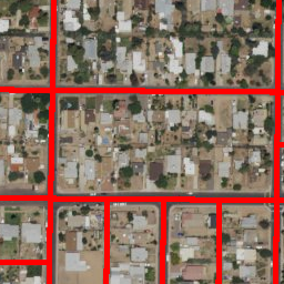Figure 3. Left: Road labels in red without dilation. Right: Twice dilated.

Although road labels are produced for all images, only data corresponding to the Phoenix, AZ area are used for training and evaluating the CNN performance. Since the Phoenix area is rather large and neither images nor labels can comfortably fit in 16GB of memory, the Phoenix data is split into Training/Development/Testing partitions and exported to an HDF5 dataset. In total, there were 16128 512x512-pixel RGB images separated into a 12864/1632/1632 train/development/test split (80/10/10% split).

Preprocess

For implementing the perimeter detection procedure, it is convenient to have a single image that encompasses a city rather than multiple smaller images. In this step, the GDAL program is used to mosaic the multiple images previously downloaded into a single georeferenced image for each city (as in Figure 1a).

Learn

The aerial images and respective labels corresponding to the Phoenix, AZ area were previously organized into 12864/1632/1632-sized training/development/test sets in the Labels section.

A modified U-Net CNN architecture was fit to the training set with performance metrics evaluated on the development set for refinement. The dice coefficient was used as the loss function but other metrics such as cross entropy, precision, and recall were also calculated. The architecture here is very similar to the original U-Net but with added dropout and batch normalization layers, summation skip connections rather than concatenation, and learnable transpose convolution layers instead of static upscaling. The layer-by-layer summary is reported in the Jupyter notebook as are final performance metrics evaluated on the unused test set.

The CNN takes as input a 640x640x3-pixel RGB image and produces a 512x512x1 image with pixel values corresponding to the probability of that pixel containing a road. To account for the height and width difference between input and output, a raw 512x512x3 input is first padded with 64-pixel reflections on each side to produce the 640x640x3 input. The final 512x512 output corresponds to the original 512x512 input dimensions.

The model was implemented via the Keras library with Tensorflow GPU backend.

Predict

The CNN trained in the previous section was applied to five Arizona cities: Bullhead, Lake Havasu, Flagstaff, Globe, and Yuma. For each city, the mosaic created in the preprocessing step was split into 512x512x3 tiles each of which were then padded with 64-pixel reflections on every side to form the 640x640x3 inputs needed. The resulting prediction tiles were rearranged back into a single image roughly the same size as the original mosaic (see Figure 1b); some pixels were cropped off the mosaic to ensure it could be evenly divided into the 512x512-pixel tiles.

Image Processing

The prediction images in the last step were rounded to produce a single binary mask for each city with pixel values of 1 indicating the presence of a road and 0 otherwise. Morphological operations via the OpenCV library were applied to these images.

First, the road network was expanded through a dilation operation repeated 95 times with a small 3x3 square kernel. The goal of this operation is to connect unconnected roads and make the road network into a single, completely connected mesh that surrounds the entire city. Then, an erosion with the same 3x3 kernel was applied and repeated 95 times. This ensures the boundary of the road network mesh does not exceed the bounds of the original, undilated predictions. Figure 4 shows an example application of these steps.

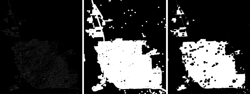
Figure 4. Morphological operations. Left: Starting road network predictions. Middle: Dilation applied. Right: Erosion applied.

After the morphological operations were applied, contours were found for all objects in the image. Often there were multiple distinct, unconnected objects, so the contour of the largest object was taken to be the city perimeter. This contour could then be overlaid on the original aerial image for visual assessment (as in the Results section).