Interactive visualization of various dimensionality reduction algorithms applied to US Congressional voting data.
Update: the interactive viz is currently unavailable.
Overview
Dimensionality reduction techniques seek to embed high-dimensional data into lower-dimensional structures. In linear algebra terms, given a fat \(m \times n\) matrix \(\textbf{X}\), they construct a new, skinny \(m \times k\) matrix \(\textbf{M}\) with \(k << n\) that preserves some of the information in \(\textbf{X}\). The lower-dimensional data is often useful as features for statistical modeling or for finding clusters in exploratory analyses.
In this project, the \(m\) rows of \(\textbf{X}\) correspond to legislators of the US Senate and House of Representatives, and the \(n\) columns each represent a bill that was voted on. The elements of \(\textbf{X}\) are thus filled with the legislators’ votes on the bills such as ‘Yea’ or ‘Nay’ (technically, the columns are then one-hot encoded; see Methods). Various embedding algorithms are applied to generate multiple embedding matrices \(\textbf{M}\). We choose to generate \(k = 3\) columns of \(\textbf{M}\) in order to visualize the results in two and three dimensions.
Results
Most of the embedding algorithms produce two distinct structures:
- Democrat / Republican split
- House / Senate split
The second point is somewhat artificially induced. Each of the original columns \(\vec{x_i}\ (i \in [1 \ldots n])\) of \(\textbf{X}\) correspond to a bill in the House or Senate, but the \(m\) rows (i.e. the length of \(\vec{x_i}\)) represent legislators in both the House and Senate. Thus, if \(\vec{x_i}\) corresponds to a bill in the House, all the senators’ votes are filled with a null code. This creates a strong pattern for all senators and a complementary pattern for representatives. Although this could be avoided by applying the embedding algorithms separate for the house and senate, it is a useful pedagogical quirk and thus kept for this project. See the Methods section for full vote encoding details.
The first point is more interesting and reflective of real voting patterns: Republicans vote with Republicans and Democrats with Democrats, and they usually don’t agree. The trend is so strong that in many instances the Democrat and Republican clusters are almost linearly separable.
We can compare legislators known to buck party trends and see they do indeed lean toward the opposite party cluster. Based on data from this Washington Post article, some of the top party outliers are Collin Peterson, Kyrsten Sinema, Brad Ashford, Henry Cuellar, and Jim Costa for House Democrats and Christopher Gibson, Robert J. Dold, Carlos Curbelo, Richard Hanna, Ileana Ros-Lehtinen, Michael Fitzpatrick, and Frank LoBiondo for House Republicans. All the mentioned representatives trend toward the opposite party House clusters as shown for the 2016 session below.
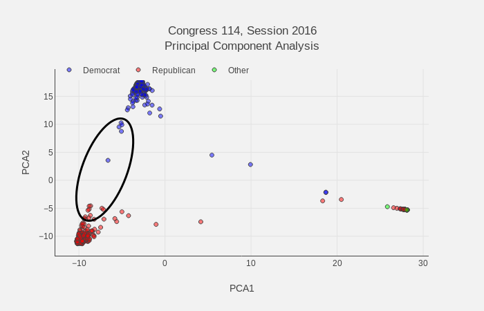
Legislators that often vote against their party trend toward opposite party clusters. The black ellipse encompasses the most prevalent party buckers within the House.
Conclusion
Based only on voting records, we have shown that dimensionality reduction algorithms can detect the Democrat/Republican party split that dominates the US Congress. Additionally, many of the embeddings are capable of incorporating nuance into their structures such as embedding legislators that buck the party trend toward the opposite party. The results are displayed interactively to facilitate exploratory analyses.
Methods
Full source code is available on GitHub.
Congressional voting data for session years 2009 - 2017 were downloaded with this scraper. Only votes consisting of ‘Yea’, ‘Nay’, ‘Aye’, ‘No’, and ‘Not Voting’ were considered; this eliminated a few (\(< 50\)) votes such as votes for electing Speaker of the House. The ‘Yea’ and ‘Aye’ votes were coded to ‘Yes’, ‘Nay’ and ‘No’ to ‘No’, and ‘Not Voting’ to ‘Neutral’. For each year individually, these votes were arranged in a matrix with rows and columns corresponding to legislators and bills, respectively. The number of bills (i.e. features) per year ranged from 783 to 1383.
Since each bill was voted on only in one chamber of Congress, but the rows are comprised of legislators from both chambers, an additional ‘NaN’ code was used to fill rows representing senators in House votes and similar for representative in Senate bill votes. The ‘Yes’, ‘No’, ‘Neutral’, and ‘NaN’ votes were then one-hot encoded to produce the final matrix for embedding. We note that the use of categorical variables for some of these algorithms may be somewhat dubious theoretically, but they often do produce useful and interpretable results as done here, so the encoding scheme has practical merit at least.
Scikit-learn implementations of the following dimensionality reduction algorithms were used:
- Principal component analysis (PCA)
- Multidimensional scaling (PCA)
- Spectral Embedding (SE)
- t-distributed Stochastic Neighbor Embedding (TSNE)
- Isomap (ISOMAP)
The algorithms were applied to each year of data separately. Default parameters were generally used for each algorithm, but exact parameters can be found in the source code.
The interactive visualization was produced with the Dash framework. Metadata for the visualization such as party and state affiliation were sourced from this repository.